Since the beginning of my doctoral research, through my work as a research scientist, I have been using and helping develop Lagrangian techniques, some better known than others. Here I give brief descriptions of some of these methods.
Lagrangian label technique
The Lagrangian label technique is a powerful method providing a rather complete characterization of fluid motion. This method was an idea of Professor John S. Allen (personal communication) and was first published in Kuebel-Cervantes et al. (2003). To my knowledge, only a handful of papers have used this technique so far, despite its usefulness.
In the Lagrangian view, water parcels are followed along their paths, it is therefore necessary to give each parcel a unique identity. A natural option is to label parcels with their initial position. The Lagrangian label technique uses three passive tracers, one for each coordinate in three-dimensional space, with the initial condition for each parcel being the coordinates of each parcel’s grid cell. So, for example, the label X is a passive dye representing the longitude of each water parcel at it’s initial position: X(x,y,z,t=0)=x . The labels for latitude and depth have similar initial conditions: Y(x,y,z,t=0)=y and Z(x,y,z,t=0)=z . The numerical simulation of fluid flow then begins, and with the velocity, the Lagrangian labels are advected as conserved quantities: \frac{D}{Dt} (X,Y,Z)=(0,0,0) . Here is a plot of the three dyes at time zero: 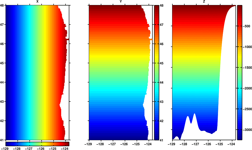
The left panel is the longitude label X and the middle panel is the latitude label Y, both are plotted at a constant depth as a function of longitude and latitude, notice the colorscale is the same as the x-axis for the longitude label, and equal to the y-axis for the latitude label. This initial condition is the same at each depth. The panel on the right is the initial condition for the depth label Z plotted at a constant latitude, as a function of depth and longitude; the colorscale is equal to the z-axis. This initial condition is the same at each latitude.
Using a realistic ROMS simulation off the U.S. west coast, here are the labels at a fixed depth z=250m, after a month advection initialized on July 1, 2005: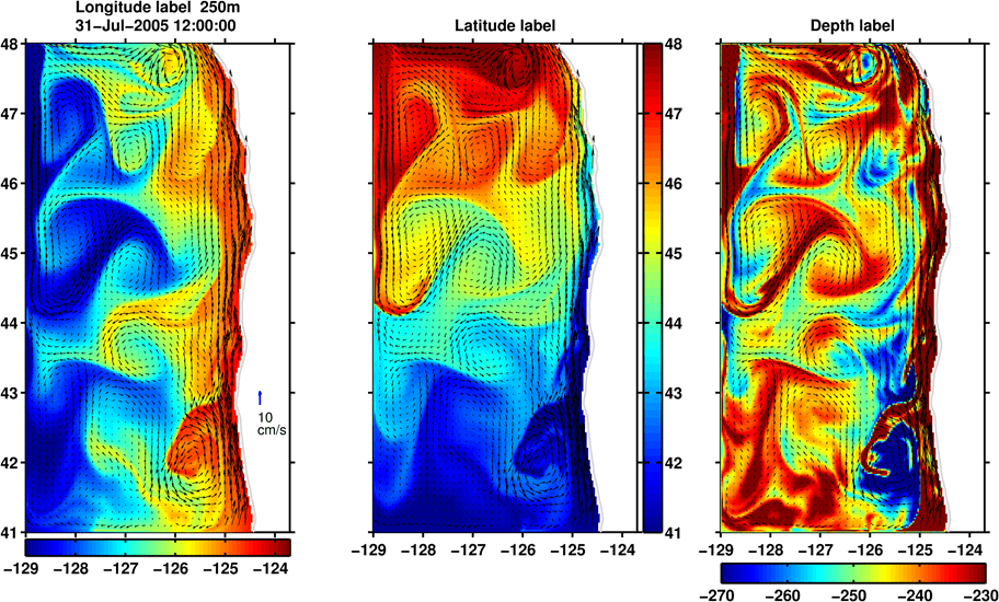
The poleward undercurrent is evident next to the slope in the Eulerian velocity (vectors) and the Latitude label (middle panel). The Longitude label (left panel) shows the undercurrent losing water offshore (e.g. ~42.5^\circN and 46^\circN), and some limited entrainment in the outer part of the undercurrent: yellow tracer, which represents an initial longitude of about X=-125.8, can be seen joining the outer part of the undercurrent between 41–42.5^\circN. The depth label (right panel) shows that downwelling (20+m over a month, roughly 1 meter per day) is pervasive through the meridional extent of the domain (which is the meridional extent of the undercurrent) next to the bottom, suggesting offshore Ekman flow through bottom friction.
The Lagrangian Label technique gives a useful three-dimensional Lagrangian characterization of flow. For this method, physical diffusion should be turned off, however, numerical diffusion will limit the span of useful integration. In my experience, the Lagrangian label technique gave meaningful results over monthly periods without concern for the grid size (numerical Peclet number) or numerical advection scheme—it is possible one can extend the period further. A variety of analyses can be done with this method, some of which can be seen in chapter 2 of my dissertation. A similar application of the method can be seen here in a very cool animation of an eddy.
References
Kuebel Cervantes, B. T., J. S. Allen, and R. M. Samelson (2003), A modeling study of Eulerian and Lagrangian aspects of shelf circulation off Duck, North Carolina, Journal of Physical Oceanography, doi:10.1175/1520-0485(2003)033<2070:AMSOEA>2.0.CO;2.