The motivation behind this project was seeking dominant Lagrangian transport patterns while bypassing the chaos inherent to trajectories in geophysical flows, which are rich in quasi-geostrophic turbulence. A relatively simple approach capitalizing on novel methods from nonlinear dynamics has proved fruitful, providing several developments:

— to my knowledge, it is the first way of computing proper Lagrangian climatologies (in a section below we show that previous attempts result in both accurate and spurious patterns),

— it is very effective in synthesizing Lagrangian information from vast amounts of Eulerian data

— it shows that it is possible to extract quasi-steady, general transport patterns that describe important aspects of the inherently time-dependent, chaotic problem of oceanic Lagrangian transport

— it suggests the existence of a connection between low-frequency Lagrangian and Eulerian kinematics of geophysical flows

— it shows that an Eulerian velocity climatology preserves important Lagrangian transport patterns from the instantaneous Eulerian velocity—to my knowledge, this is the first time that climatological and instantaneous Eulerian velocity fields are linked in Lagrangian terms.

— Lagrangian climatologies are effective in extracting the results obtained from many studies, all in one blow!

This post aims to exemplify these developments.

A question such as “What are the predominant transport patterns?” is often tackled by running a large number of simulations and then looking at the probability of trajectories reaching a certain region. A problem with this approach is that once you run a large number of trajectory simulations initiated at some point source, you still know nothing or very little regarding Lagrangian transport patterns originating elsewhere. Also, while this approach establishes connectivity from a point source, it does not provide much information on the pathways. Nonlinear dynamics is the right type of tool for this type of problem because instead of studying a point source, it studies the properties of the flow map. A flow map is a mapping taking all possible initial conditions within a domain to their final position along their trajectories, thus providing a complete account of Lagrangian behavior within a domain of interest. If x(t;x_0,t_0) is a trajectory that satisfies \frac{d x}{d t} = v(x,t),  given an initial condition x(t_0)=x_0, then the flow map up to time t_1 is F_{t_0}^{t_1}(x_0 ) , and it is defined as  F_{t_0}^{t_1}(x_0 ) \equiv x(t_1;x_0,t_0) \quad \forall x_0  \in U \subset \mathbb{R}^2 (for all possible initial conditions within a domain, in this case a subset of the cartesian plane).

Now if we are interested in general, persistent transport patterns, then we are not interested in a flow map that depends on some choice of initial and final times t_0 and t_1. Fortunately, approach zero (i.e. average and see what happens) turned out to be a very good way of bypassing this dependence. Two types of averaging are used. Perhaps in the future, I will write a post discussing why this works, what are the implications, and what type of future work this suggests.  The result is that the method does indeed find persistent transport patterns that do not depend sensitively on when or where a trajectory initiates or ends.

Thanks to work with collaborators around the world, we now know that the method is robust in the sense that it gives very good results whether using free-running numerical ocean models, or data-assimilating models. Also, the method works well under different regional oceanographic settings. The method has been used in three different Gulf of Mexico studies, in the Red Sea, off the coast of Brazil, in the subtropical Atlantic, in the Caribbean Sea, and the Arabian Sea. Results from each of these projects are presented here, including figures that can’t always make it to publications, but that help tell an important part of the story.

Reading the freely available paper where the method is developed is a good place to start, it should be a relatively quick read: https://www.nature.com/articles/s41598-018-23121-y.

The code is also freely available if you’d like to try it out; you can, for example, replicate the results of the paper above. A modern laptop can compute the same 12-month Lagrangian climatology for the Gulf of Mexico in about 2 hours, there are detailed instructions in the README.md file: https://bitbucket.org/rodu/clcss/src/master/

Before we start, I would like to acknowledge the generous funding that made this possible, from the U.S. Department of Energy, National Energy Technology Laboratory. This work is the backbone of the Climatological Isolation and Attraction Model (CIAM), a component of the Offshore Modeling Suite that is being used in different parts of the world.

Introduction

When computing a Lagrangian climatology, one obtains climatological Lagrangian Coherent Structures (cLCS) and their strength of attraction ( c \rho ). In their supplemental information, Duran et al. (2018) showed that monthly cLCS are effectively equivalent to the superposition of Lagrangian Coherent Structures from the dynamical systems in the corresponding month when computed with the climatological velocity. (Each choice of t_0 and t_1 determines a unique finite-time dynamical system.) This means that monthly cLCS and their strength of attraction are similar to any LCS, and their strength of attraction, within that month. In other words, although not formally preserved, LCS properties such as impeding transport, and deforming with transport,  tend to hold with cLCS as well although I note that these are Lagrangian properties for the climatological circulation. Thus, the important question becomes: What does the climatological velocity have to do with transport sustained by the instantaneous velocity? In Duran et al. (2018) we showed that the ensemble-mean Lagrangian transport of the instantaneous velocity is strongly constrained by the cLCS. Equivalently, in the ensemble mean, where the averaging takes place over different initial times, the Lagrangian transport of the instantaneous velocity closely resembles LCS from the climatological velocity. This is a topic that deserves future research. Beyond what was shown in Duran et al (2018), below are further examples of how cLCS constrain observed instantaneous Lagrangian transport and modeled instantaneous Lagrangian transport. These results hold with a variety of free-running models and in different regions, suggesting something meaningful and robust has been discovered.

 

Illustrating cLCS

A couple of videos made by Dr. Justino Martínez from the Instituto de Ciencias del Mar in Barcelona offer a good illustration of how cLCS work, thus aiding in their interpretation. Blue dots are synthetic tracers moving with a climatological velocity and brown lines are cLCS for January (first movie) and August (second movie):

Some comparisons of cLCS with data and models in the Gulf of Mexico

In Gough et al (2019) it was shown that cLCS can indicate cross-shelf transport barriers. For example, in one experiment they use synthetic drifters advected with their instantaneous velocity, thus showing that 1) cLCS near the shelf accurately indicate transport barriers and 2) the climatological velocity preserves dominant transport patterns from the instantaneous velocity.

Persistent transport barriers and cross-shelf transport

In the following figure, color indicates the tracer density from synthetic drifters released from the black square and advected with the instantaneous velocity for 7, 14, and 28 days in January, July, April, and October. The percentage in the bottom right of each panel is the percentage of tracer crossing cLCS, as represented by the magenta dashed line. Black and gray lines are cLCS.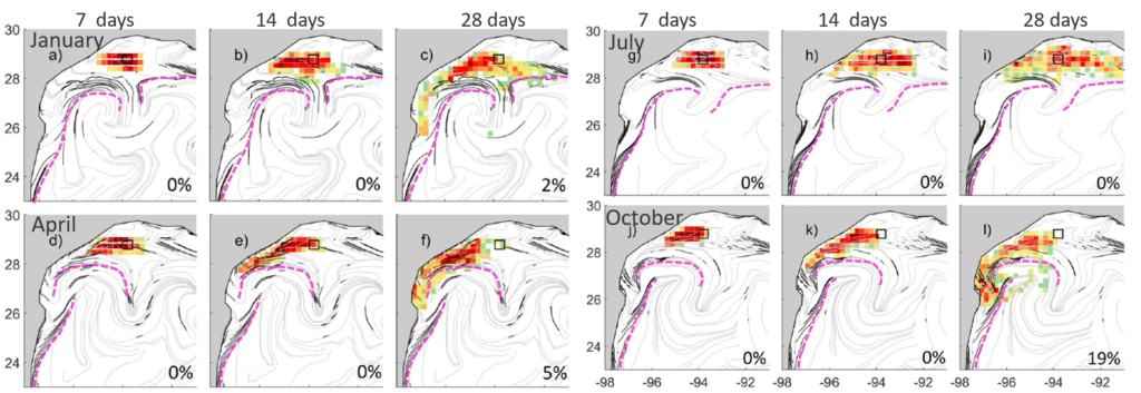

Credit Gough et al (2019)

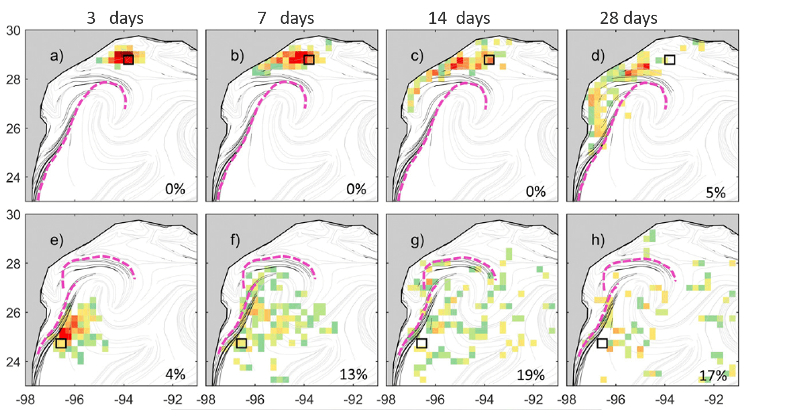
The next figure is the same as the previous but with synthetic trajectories initiated outside of the shelf (in the black square):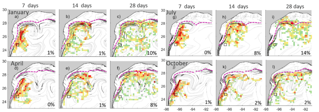

Credit Gough et al (2019)

In another experiment,  Gough et al (2019) confirm that the hook-like cLCS are indeed transport barriers in the ocean, by using over 3200 satellite-tracked drifters spanning 23 years (1994–2016), as can be seen in the following figure. Color is again drifter density, black and gray lines are now annual cLCS (rather than monthly) in all panels:

Credit Gough et al (2019)

Notice that Duran et al. (2018) found the same type of transport barriers (hook-like cLCS) using an operational HyCOM simulation, while Gough et al. (2019) use a free-running NEMO simulation.

The above figures show that the Louisiana-Texas (LaTex) shelf is isolated, which is what Duran et al. (2018) claimed for all three wide shelves in the GoM.  So what about the Yucatan shelf? Beyond the evidence in Duran et al. using satellite images from the Ixtoc oil spill, here is additional evidence from plotting all the drifters in the GoM over 27 years, the following figure was prepared by Jonathan Lilly:

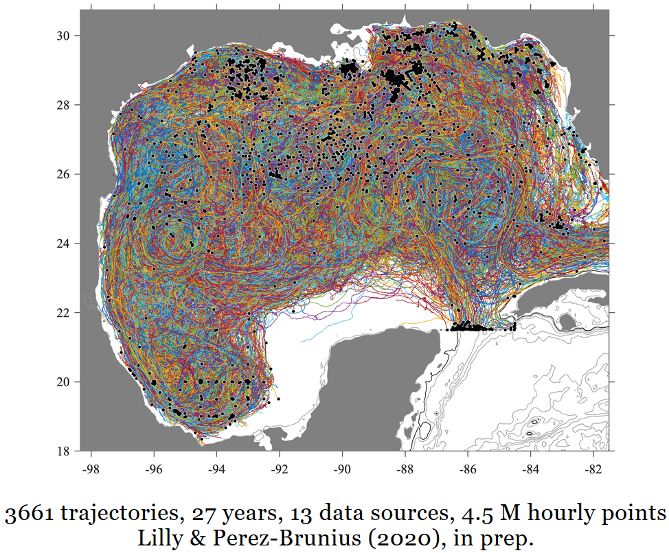
Credit: http://jmlilly.net/talks/lilly20-os/index.html#2

From the previous figure, one might ask what happened to isolation within the LaTex and West Florida shelves? Well, this figure cannot be used to assess isolation for these shelves because many drifters were released within them—the black dots are the release positions.

Finally, let’s show proof beyond that presented in Duran et al. (2018) for the isolation of the West Florida Shelf with a plot of 23 years of data released near, but outside the WFS:

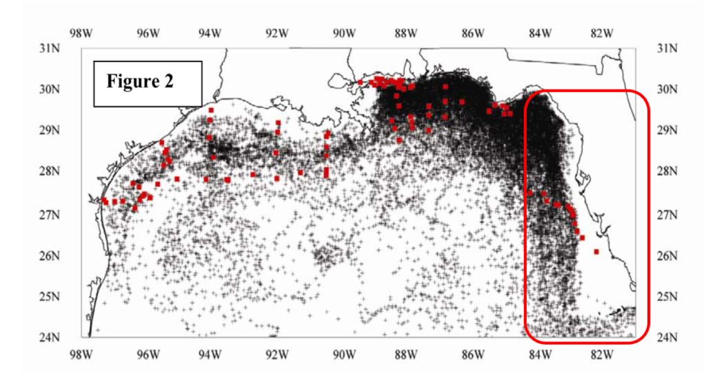
Credit:  Johnson 2008

The transport barrier isolating the WFS can be seen in the drifter data (black dots are almost 78,000 daily positions, red dots are ADCP locations), and is relatively well documented (Olascoaga et al. 2006, Olascoaga 2010).

The climatological strength of attraction c \rho is also an informative quantity. It may also identify transport barriers, for example, Greer et al. (2018) found that tracer does not reach the Mississippi coast (just east from the Mississippi delta) in fall (October), but does reach the coast in spring (April), here is one of their figures:

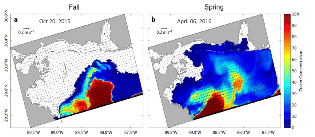
Credit Greer et al (2018)

Such patterns are anticipated by the c \rho computed in Duran et al. (2018). In October (left panel)  a c \rho maxima (color) aligns the 50-m isobath (blue line) indicating a transport barrier, inshore from this barrier c \rho is mainly weak indicating stagnation, in April (right panel) however, the transport barrier opens and even aligns perpendicular to the coast indicating persistent cross-shelf transport (indicated by a black arrow):

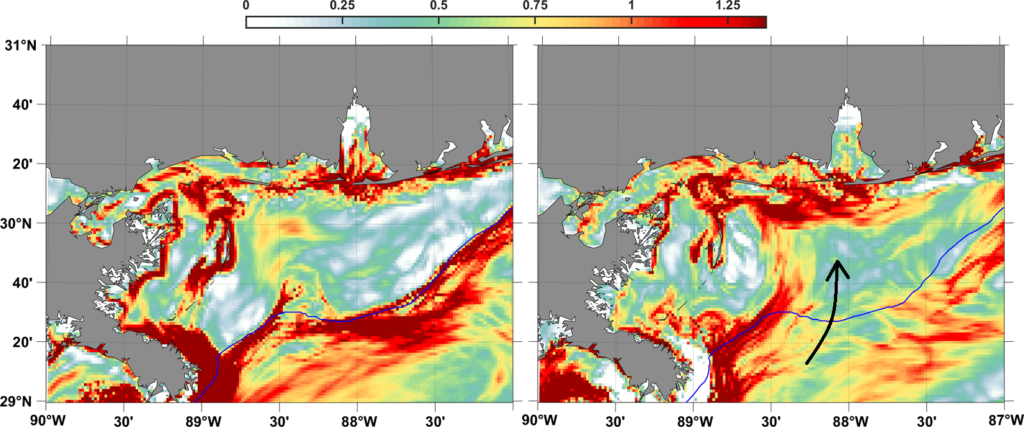
Notice the black arrow aligns with the tracer maxima in Greer et al (2018); two different models and approaches coinciding in a location for persistent cross-shelf transport.
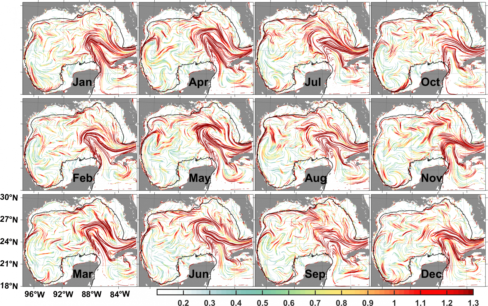
While Greer et al. (2018) obtained an interesting result which is valid for spring 2015 and fall 2016, the Gulf of Mexico Lagrangian climatology found by Duran et al. (2018) provides generalized results: likely transport patterns in any given month. The Lagrangian climatology accurately anticipates that cross-shelf transport just east of the Mississippi delta (29–30^circN, 87–89^circW) goes through an annual cycle. It is relatively isolated in the winter (left column) and fall (right column), when c \rho shows a cross-shelf transport barrier aligned with isobaths, similar to October in the figure above. In spring and summer (middle columns) not only does the shelf become a region of maximal attraction (high values of c \rho are now prevalent over the shelf), but also the transport barrier “opens”, aligning normal to isobaths, similar to the figure for April above:

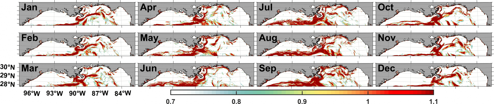
Notice the white within the WFS and the LaTex shelves, this is the isolation of large shelves, as seen through the values of c \rho . The reason low c \rho can imply isolation is because straining and shear are minimal relative to other regions in the domain, making it unlikely that trajectories ending within the shelves would have originated outside, or that trajectories ending outside would have originated from inside.  This interpretation is supported by the fact that cross-shelf flow is unlikely in geophysical fluids due to the conservation of vorticity.

These results also agree well with several other studies: should there be a spill, the Mississippi delta and the coastline to the east up to Florida is most at risk of contamination in spring (Ji et al. 2011, Barker 2011, Tulloch et al 2011), which is indeed what happened during the Deepwater Horizon accident that began in late April and lasted 5 months. In the following figure from observations, the red coastline indicates maximum oiling, yellow intermediate, blue without oil, and gray means limited tarballs:

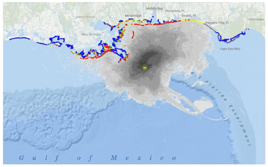
http://gomex.erma.noaa.gov

Thus, beyond transport barriers, cLCS can also indicate dominant transport patterns, including regions of enhanced cross-shelf transport and coastal vulnerability when the strength of attraction is high near the coastline. Let’s give additional examples on coastal vulnerability followed by examples of cross-shalf transport.

Coastal vulnerability in the Louisiana-Texas shelf

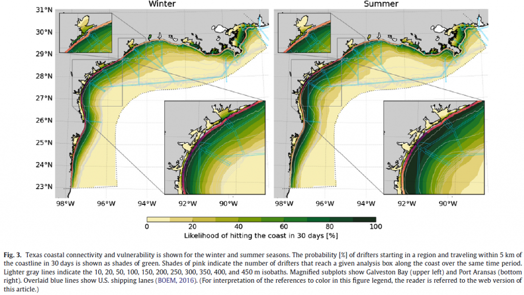
Thyng & Hetland (2016) use numerical simulations to identify the vulnerability of the Louisiana-Texas shelf in terms of pathways for oil, or other hazardous material, ending near the coastline. They find a strong attraction along the coastline (dark green means a higher probability of trajectories reaching that location) in both winter and summer, although the coastline between about 92W and 94W is less vulnerable than west of 94W or near the Mississippi delta region (east of 92W).

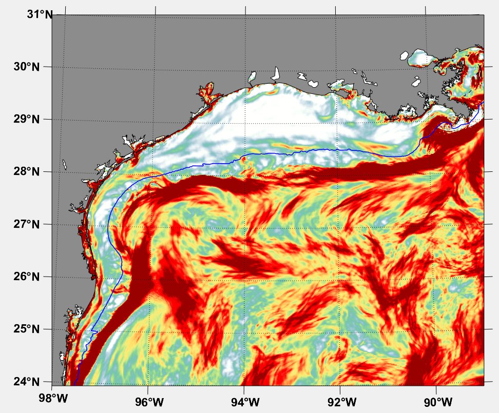
This is consistent with strong persistent attraction (the c \rho computed in Duran et al. 2018) as seen in, for example, January:

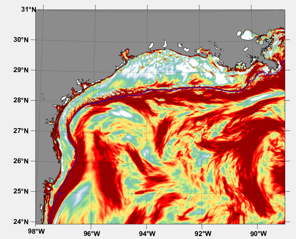
And, as another example, in August:

Persistent or recurrent trajectories including more cross-shelf transport examples

Martínez-López &  Zavala-Hidalgo (2009) uses 11 years (1997–2007) of satellite imagery to detect recurrent cross-shelf transport patterns at three GoM locations, the Perdido region around 26N next to the Gulf’s western boundary, around 92W in the southern Gulf’s boundary (Bay of Campeche) and offshore from the Mississippi delta region. These transport patterns can be clearly seen in their figure 5 (shown next), monthly chlorophyll anomaly for July, August, September, and October: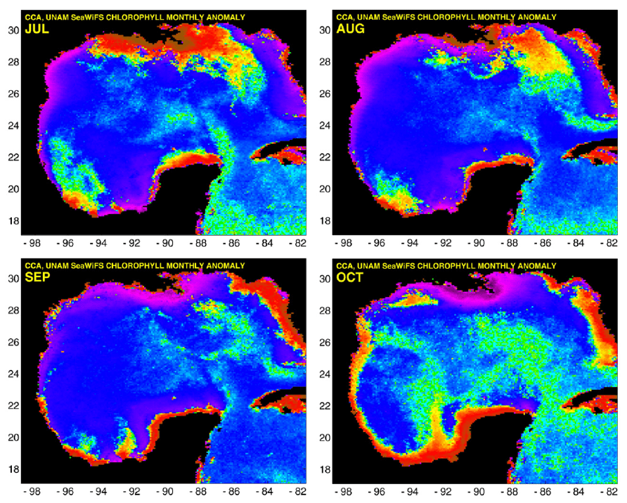

Credit: Martínez-López & Zavala-Hidalgo et al (2009)

They also found that these offshore transports have maxima in November–December (Bay of Campeche), in May (Perdido), and in June–July (Mississippi delta):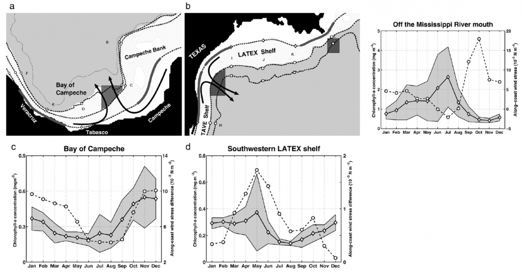

Credit: Martínez-López & Zavala-Hidalgo et al (2009)

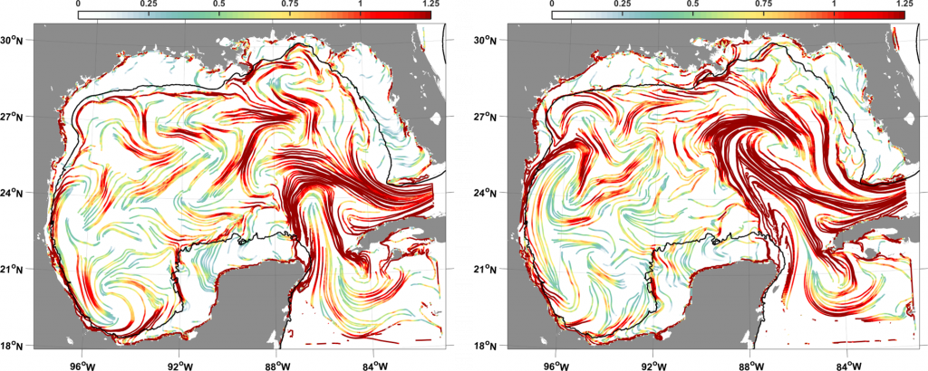
cLCS pick up these patterns precisely in time and location. November cLCS (left panel in next figure) show the clear Bay of Campeche offshore transport, but not much offshore transport in Perdido. May cLCS (right panel in next figure) clearly show strong offshore transport in Perdido but not much going on in the Bay of Campeche, note that the offshore transport near the Mississippi delta in May (not so much in November) is also accurate in time and space:

The next unpublished example further confirms that cLCS also get the Mississippi delta offshore transport accurately, along with other predominant pathways that have been found in the region.  Androulidakis et al. (2018) found three dominant patterns off the Mississippi delta, during April–June (left column),  the same three patterns are indicated by cLCS (right column shows cLCS for April and May, June is similar but not shown):

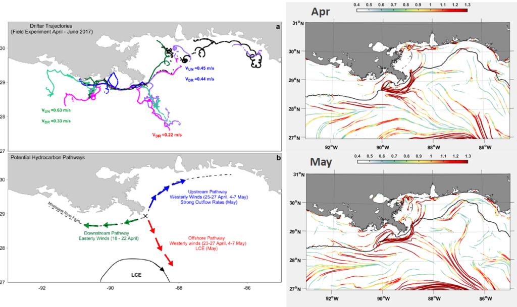
Credit Androulidakis et al (2018)

Indeed in Duran et al (2018) it was noted that in May and July the offshore transport pattern that has been observed often is very accurately depicted by cLCS (above May cLCS agree with oil from Deepwater Horizon, below July cLCS agree with drifters):

 

Trajectories from another model at a deep horizontal section

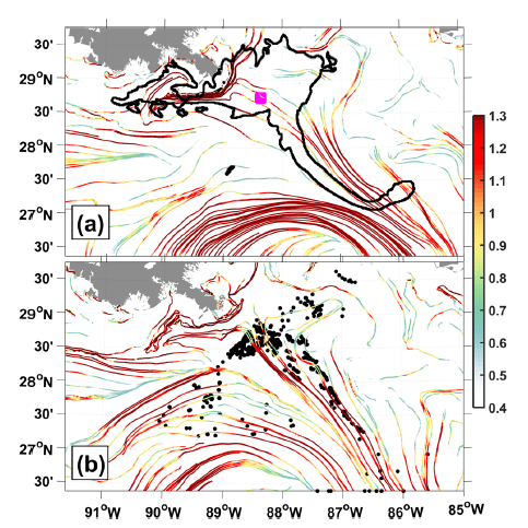
For another example of dominant transport patterns, let’s move on to the deep Gulf of Mexico (1500–2500 m). Maslo et al. (2020) found an excellent agreement between synthetic drifters advected with the instantaneous velocity from a free-running ROMS simulation, and cLCS and  c \rho (right panel) from the same model (they call them differently but they are the same thing):

Credit Maslo et al (2018)

These patterns are also in excellent agreement with the circulation documented by 158 RAFOS floats parked at that depth, between 2011 and 2015:

Credit Maslo et al (2018)

Thus, once again a Lagrangian connection is made between the instantaneous Eulerian velocity and the climatological Eulerian velocity, and once again a connection is made between the cLCS of a free-running model and observations.

What about other ways of computing a Lagrangian climatology?

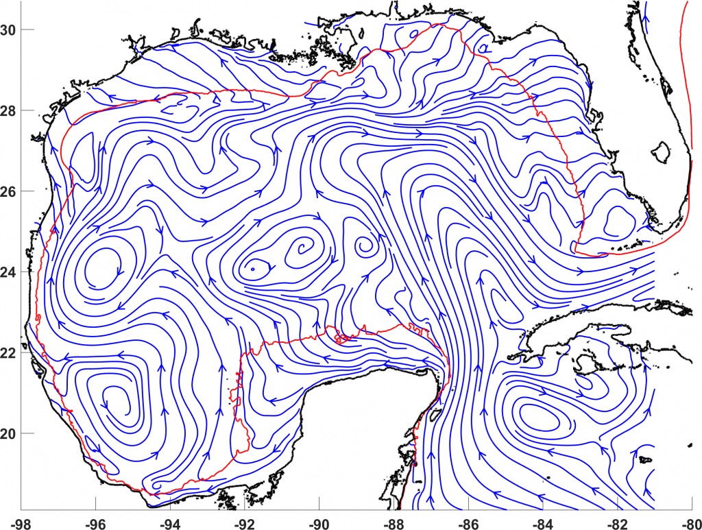
Going back to the surface of the GoM, Jonathan Lilly presents an interesting figure—the left panel is a carefully time-averaged pseudo-Eulerian velocity from all drifters in the Gulf of Mexico over 27 years, the right panel is the streamlines from this pseudo-Eulerian velocity:

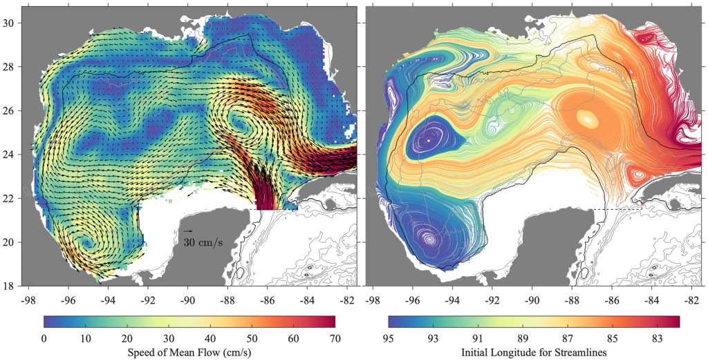
Credit: Jonathan Lilly http://jmlilly.net/homepage/2020/02/14/gulf-of-mexico-currents.html

Notice that for a time-independent flow, streamlines are the LCS, so the right panel can be compared to cLCS. There are several similarities with the quasi-steady transport patterns extracted with cLCS (next figure), for example, westward flow between 96–90^circW and 22–24^circN, that turns northward as it approaches the coast near  96^circW, and then moves offshore near 26^circN (the offshore turn is the hook pattern studied in Gough et al. 2019). The cyclonic circulation between 96–92^circW and 18–22^circN is also consistent in both figures. However, notice how the streamlines in the right panel of the figure above approach the coast with a considerable normal-to-the-coast component in Florida’s panhandle coast, in the west Florida shelf, and in the Louisiana-Texas shelf. Since trajectories must be along the streamlines of a time-independent velocity, this indicates unrealistic cross-shelf transport.

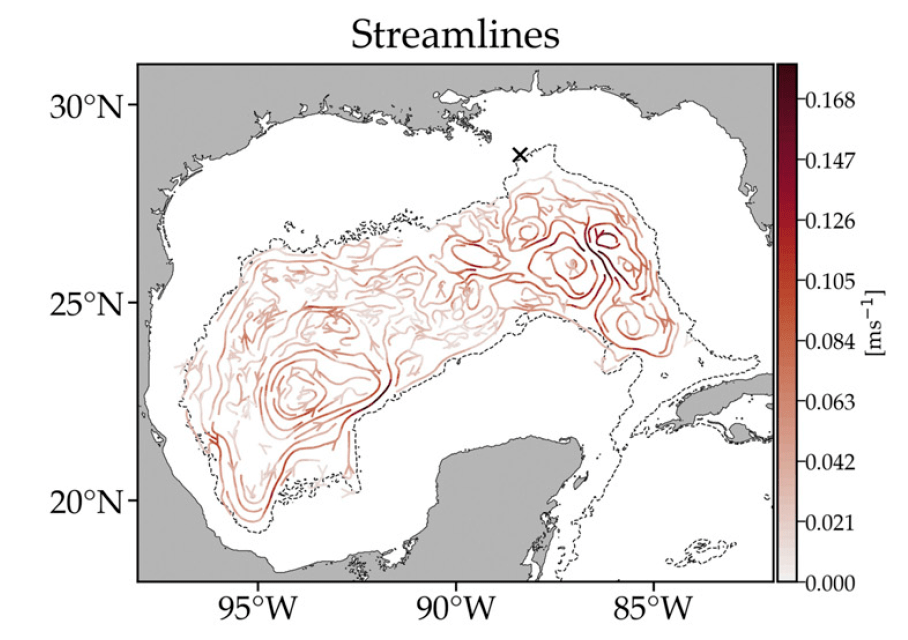
Streamlines indicating unrealistic cross-shelf transport from a time-averaged Eulerian velocity were also noted in the supplemental information of Duran et al. (2018). For example, the following figure shows the streamlines of the climatological velocity used in Duran et al. (2018) after monthly averaging over April. A very similar figure emerges when compared to the streamlines from Lilly above, including the unrealistic cross-shelf transport. These examples illustrate the problems that can happen with some types of Eulerian velocity averaging.

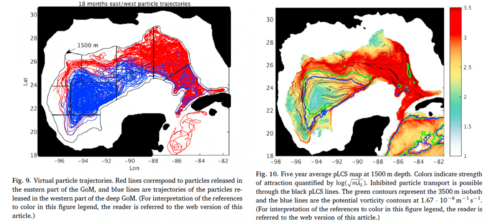
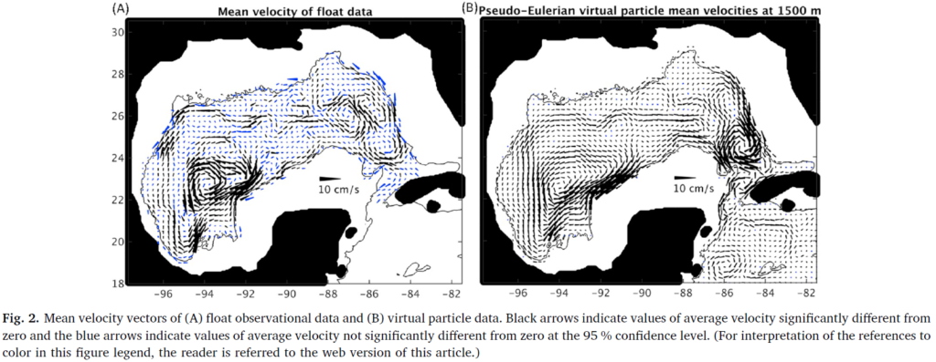
To show a different example of how streamlines from time-averaged Lagrangian observations give spurious results, we return to the deep (~1500m) GoM. The next figure shows streamlines from float data (deep drifters, see the figure by Maslo et al. 2018 above):

Credit: Miron et al. (2019).

A tracer can be advected with this velocity, and the circulation does not resemble the trajectories from which the streamlines were obtained!

Credit: Miron et al. (2019).

And the results do not improve when adding eddy diffusion either:

Credit: Miron et al. (2019).

These examples show that not just any averaging of the Eulerian velocity—or even any averaging of Lagrangian data—is adequate for Lagrangian climatologies. The trajectories from some averaged fields have spurious artifacts.

Regional Examples

The following presentation by Dr. Justino Martínez from the Instituto de Ciencias del Mar in Barcelona gives some insights into the work being done in the Mediterranean and Iberian Atlantic, with some interesting examples of preliminary findings:

To be continued (work in the Mediterranean, Iberian Atlantic, Red Sea, North Sea, Bay of Bengal, Caribbean Sea, Equatorial Atlantic has not been added yet!)…

 

References (peer-reviewed papers developing or applying cLCS are bold):

• Duran, R., F. J. Beron-Vera, M. J. Olascoaga (2018). Extracting quasi-steady Lagrangian transport patterns from the ocean circulation: An application to the Gulf of Mexico. Scientific Reports, 8(1), 5218. https://www.nature.com/articles/s41598-018-23121-y
• Gough M. K., F. J. Beron-Vera, M. J. Olascoaga, J. Sheinbaum, J. Jouenno, R. Duran (2019). Persistent Lagrangian transport patterns in the northwestern Gulf of Mexico. J. Phys. Oceanogr., 49, 353–367, https://doi.org/10.1175/JPO-D-17-0207.1
• Greer, A.T., et al. (2018). Functioning of coastal river-dominated ecosystems and implications for oil spill response: From observations to mechanisms and models. Oceanography 31(3):90–103, https://doi.org/10.5670/oceanog.2018.302.
• Androulidakis, Y., Kourafalou, V., Ozgokmen, T., Garcia-Pineda, O., Lund,B., Le Henaff, M., et al. (2018). Influence
  of river-induced fronts on hydrocarbon transport: A multiplatform observational study. Journal of Geophysical Research: Oceans, 123, 3259–3285. https://doi.org/10.1029/2017JC013514
• Maslo, A., Azevedo Correia de Souza, J. M., Andrade-Canto, F., & Rodríguez Outerelo, J. (2020). Connectivity of deep waters in the Gulf of Mexico. Journal of Marine Systems. https://doi.org/10.1016/j.jmarsys.2019.103267
• Johnson, D. R. (2008). Ocean Surface Current Climatology in the Northern Gulf of Mexico. Technical Report. https://gcrl.usm.edu/user_files/Donald.Johnson.NGOM.currents.pdf
• K. Thyng, R. Hetland (2016). Texas and Louisiana coastal vulnerability and shelf connectivity, Marine Pollution Bulletin. http://dx.doi.org/10.1016/j.marpolbul.2016.12.074

• Olascoaga, M. J., Rypina, I. I., Brown, M. G., Beron-Vera, F. J., Koçak, H., Brand, L. E., et al. (2006). Persistent transport barrier on the West Florida Shelf. Geophysical Research Letters. https://doi.org/10.1029/2006GL027800
• Olascoaga, M. J. (2010). Isolation on the West Florida shelf with implications for red tides and pollutant dispersal in the Gulf of Mexico. Nonlinear Processes in Geophysics. https://doi.org/10.5194/npg-17-685-2010
• Martínez-López, B. & Zavala-Hidalgo, J. (2009).  Seasonal and interannual variability of cross-shelf transports of chlorophyll in the Gulf of Mexico. Journal of Marine Systems 77, 1–20, https://doi.org/10.1016/j.jmarsys.2008.10.002
• Miron, P., Beron-Vera, F. J., Olascoaga, M. J., Sheinbaum, J., Pérez-Brunius, P., & Froyland, G. (2017). Lagrangian dynamical geography of the Gulf of Mexico. Scientific Reports. https://doi.org/10.1038/s41598-017-07177-w
• Gouveia, M. B., R. Duran, J. A. Lorenzzetti, A. T. Assireu, R. Toste, L. P. de F. Assad and D. F. M. Gherardi (2021). Persistent meanders and eddies lead to quasi-steady Lagrangian transport patterns in a weak western boundary current. Scientific Reports, 11(1), 497. https://www.nature.com/articles/s41598-020-79386-9
•  Allende-Arandía, M. E., Duran, R., Sanvicente-Añorve, L., & Appendini, C. M. (2023). Lagrangian Characterization of Surface Transport From the Equatorial Atlantic to the Caribbean Sea Using Climatological Lagrangian Coherent Structures and Self-Organizing Maps. Journal of Geophysical Research: Oceans, 128(7), e2023JC019894. https://doi.org/10.1029/2023JC019894